8.6. Visualization

8.6.1. RR Tachogram #

Graph of RR intervals over time:

• Blue line: RR intervals
• Gray points: local minima (respiratory cycles)
• Green line: signal power (scaled)
• Gray vertical lines: section markers

8.6.2. RR Tachogram Spectrum #

FFT spectrum of the interpolated RR signal:

• X-axis: frequency (0–0.5 Hz)
• Y-axis: spectral amplitude
• LF (0.04–0.15 Hz) and HF (0.15–0.4 Hz) ranges are marked
• LF%, HF%, and LF/HF ratio are displayed

8.6.3. Poincaré Plot (Local Return Map) #

Scatter plot of RR(i) versus RR(i-1) or RR(i-shift):

• Each point: a pair of consecutive RR intervals
• Colors: different sections
• Ellipses: 2SD1 and 2SD2 for each section

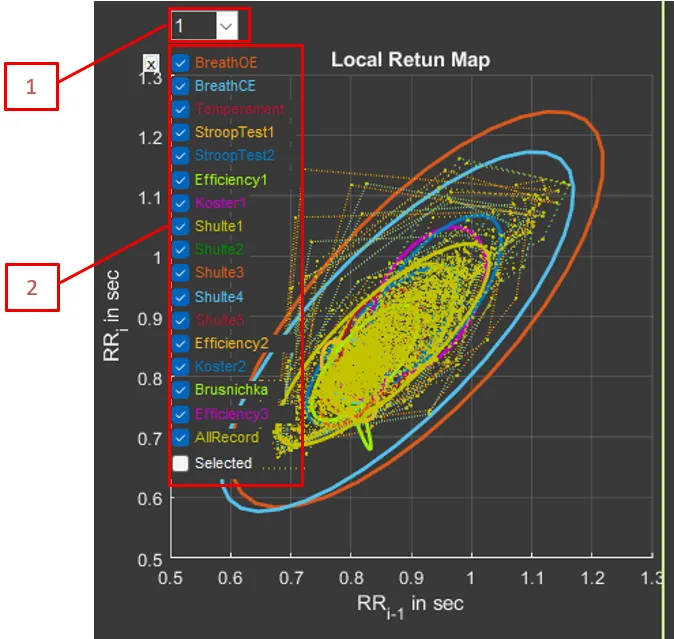
1. Shift RR: shift for the Poincaré plot (1–15 intervals)
2. Checkboxes for including or excluding sections

Physiological explanation of the Poincaré plot:

The Poincaré plot (return map) is a graphical way to visualize heart rate variability by showing the patterns of RR interval changes.

How to read the plot:

• Each point = a pair of consecutive RR intervals
• X-axis: RR(i-1), the previous interval
• Y-axis: RR(i), the current interval
• If the heart beat like a metronome, all points would be in one place.

Typical shapes:

Round/oval shape (healthy heart):

• high variability
• good adaptability
• healthy ANS state
• SD1 and SD2 are roughly equal

Elongated shape along the diagonal:

• low short-term variability (small SD1)
• long-term trends remain (larger SD2)
• possible stress or fatigue
• low SD1/SD2

Compact cloud:

• low variability overall
• very regular heartbeat
• possible health problems
• both SD1 and SD2 are small

Shifted center:

• change in mean RR
• transition between states (rest → load)
• response to a stimulus

Physiological meaning of SD1 and SD2:

• SD1 (minor axis):
  • short-term variability
  • beat-to-beat changes
  • predominantly parasympathetic activity
  • associated with respiratory arrhythmia
• SD2 (major axis):
  • long-term variability
  • trends and slow changes
  • sympathetic + parasympathetic activity
  • associated with the baroreflex and other slow regulatory processes

Clinical significance:

• Healthy people: round or oval cloud, SD1/SD2 ≈ 0.3–0.5
• Stress: the cloud becomes elongated, SD1 decreases
• Aging: the cloud becomes more compact, both SDs decrease
• Pathology: a very compact cloud or an unusual shape

8.6.4. Segmental HRV Analysis #

The graph shows the dynamics of HRV parameters over time:

• HR: heart rate
• FuncGroup: functional group (×10)
• ExtraPoint: additional score (×100)
• z(HR): pulse z-score
• z(SD1): SD1 z-score
• z(SD2): SD2 z-score
• RMSSD: RMSSD
• Relaxation: Relaxation
• Concentration: Concentration (from EEG)
• Breath: breathing rate

All parameters are calculated in a sliding window with 75% overlap.

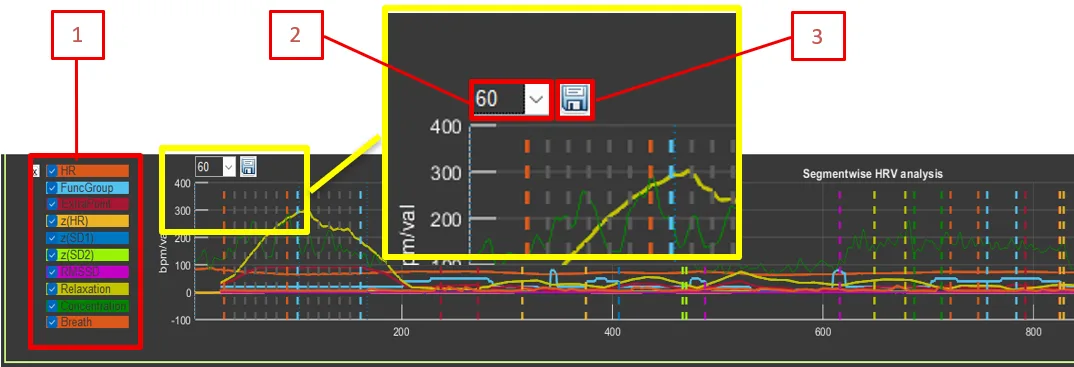
1. Checkboxes for including or excluding HRV parameters
2. Average Window: Averaging window for segmental analysis (10–100 intervals)
3. Save continuously HRV: Save continuous HRV parameters over time